simulate.blim

Simulate Responses from Basic Local Independence Models (BLIMs)

Description

Simulates response frequencies from the distribution corresponding to a fitted blim model object. Alternatively, if sufficient information is provided, it generates response frequencies from scratch (see examples).

Usage

## S3 method for class 'blim'
simulate(object, nsim = 1, seed = NULL, ...,
         method = c("bernoulli", "multinomial"), zeropad = FALSE)

Arguments

object an object of class blim, typically the result of a call to blim.

nsim currently not used.

seed currently not used.

… further arguments passed to or from other methods. None are used in this method.

method bernoulli (default) or multinomial sampling.

zeropad logical, if TRUE non-sampled response patterns have a frequency of zero, else (default) they are omitted.

Details

Bernoulli sampling: Responses are simulated in two steps: First, a knowledge state is drawn with probability P.K. Second, responses are generated by applying rbinom with probabilities computed from the model object’s beta and eta components. Faster with a large number of items.

Multinomial sampling: The probability of all response patterns is computed from the model object’s parameters, and response frequencies are obtained from rmultinom. Faster with few items but a large number of respondents.

Value

A named vector of frequencies of response patterns.

Examples

library("pks")

data(DoignonFalmagne7)
 
m1 <- blim(DoignonFalmagne7$K, DoignonFalmagne7$N.R)
simulate(m1)

00000 00001 00010 00011 00100 00101 00110 00111 01000 01001 01010 01100 01101 
   90     7     3     1     7     3     1     1    94     8    12    10    13 
01110 01111 10000 10001 10010 10011 10100 10101 10110 10111 11000 11001 11010 
   12    11   107     9    15     2    11    10     8     9    70     8    91 
11011 11100 11101 11110 11111 
    7    91   105    81   103

simulate(m1, method = "multinomial", zeropad = TRUE)

00000 10000 01000 00100 00010 00001 11000 10100 10010 10001 01100 01010 01001 
   91    97    96     6     2     6    75    10    12     8     9    16     8 
00110 00101 00011 11100 11010 11001 10110 10101 10011 01110 01101 01011 00111 
    0     1     0    69   110    15     6    10     0    14     8     2     3 
11110 11101 11011 10111 01111 11111 
  101    99     8    14     8    96

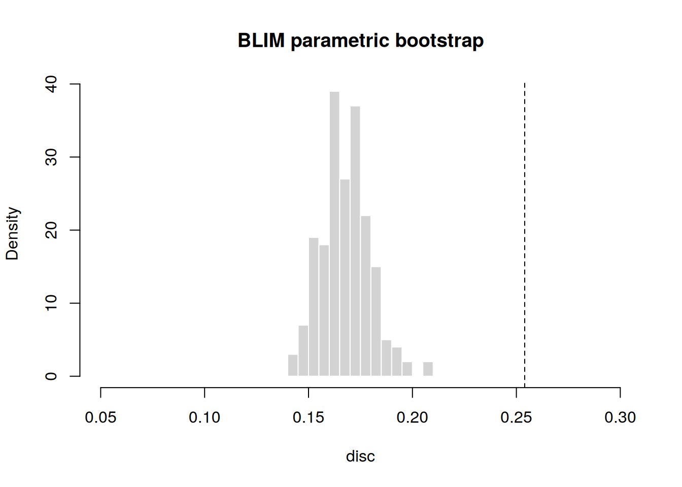
## Parametric bootstrap for the BLIM
disc <- replicate(200, blim(m1$K, simulate(m1))$discrepancy)

hist(disc, col = "lightgray", border = "white", freq = FALSE, breaks = 20,
     main = "BLIM parametric bootstrap", xlim = c(.05, .3))
abline(v = m1$discrepancy, lty = 2)

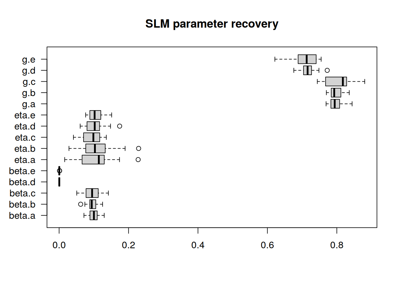
## Parameter recovery for the SLM
m0 <- list( P.K = getSlmPK( g = rep(.8, 5),
                            K = DoignonFalmagne7$K,
                           Ko = getKFringe(DoignonFalmagne7$K)),
           beta = rep(.1, 5),
            eta = rep(.1, 5),
              K = DoignonFalmagne7$K,
         ntotal = 800)
class(m0) <- c("slm", "blim")

pars <- replicate(20, coef(slm(m0$K, simulate(m0), method = "ML")))
boxplot(t(pars), horizontal = TRUE, las = 1,
        main = "SLM parameter recovery")

## See ?endm for further examples.

Code Links