Elimination-by-Aspects (EBA) Models with Order-Effect

Fits a (multi-attribute) probabilistic choice model that accounts for the effect of the presentation order within a pair.

eba.order(M1, M2 = NULL, A = 1:I, s = c(rep(1/J, J), 1),
          constrained = TRUE)

# S3 method for class 'eba.order'
summary(object, ...)

Arguments

M1, M2: two square matrices or data frames consisting of absolute choice frequencies in both within-pair orders; row stimuli are chosen over column stimuli. If M2 is empty (default), M1 is assumed to be a 3d array containing both orders
A: see eba
s: the starting vector with default 1/J for all J aspect parameters, and 1 for the order effect
constrained: see eba
object: an object of class eba.order, typically the result of a call to eba.order
...: additional arguments

Details

The choice models include a single multiplicative order effect, order, that is constant for all pairs (see Davidson and Beaver, 1977). An order effect < 1 (> 1) indicates a bias in favor of the first (second) interval. See eba for choice models without order effect.

Several likelihood ratio tests are performed (see also summary.eba).

EBA.order tests an order-effect EBA model against a saturated binomial model; this corresponds to a goodness of fit test of the former model.

Order tests an EBA model with an order effect constrained to 1 against an unconstrained order-effect EBA model; this corresponds to a test of the order effect.

Effect tests an order-effect indifference model (where all scale values are equal, but the order effect is free) against the order-effect EBA model; this corresponds to testing for a stimulus effect; order0 is the estimate of the former model.

Wickelmaier and Choisel (2006) describe a model that generalizes the Davidson-Beaver model and allows for an order effect in Pretree and EBA models.

Value

coefficients: a vector of parameter estimates, the last component holds the order-effect estimate
estimate: same as coefficients
logL.eba: the log-likelihood of the fitted model
logL.sat: the log-likelihood of the saturated (binomial) model
goodness.of.fit: the goodness of fit statistic including the likelihood ratio fitted vs. saturated model (-2logL), the degrees of freedom, and the p-value of the corresponding chi-square distribution
u.scale: the unnormalized utility scale of the stimuli; each utility scale value is defined as the sum of aspect values (parameters) that characterize a given stimulus
hessian: the Hessian matrix of the likelihood function
cov.p: the covariance matrix of the model parameters
chi.alt: the Pearson chi-square goodness of fit statistic
fitted: 3d array of the fitted paired-comparison matrices
y1: the data vector of the upper triangle matrices
y0: the data vector of the lower triangle matrices
n: the number of observations per pair (y1 + y0)
mu: the predicted choice probabilities for the upper triangles
M1, M2: the data matrices

Author

Florian Wickelmaier

References

Davidson, R.R., & Beaver, R.J. (1977). On extending the Bradley-Terry model to incorporate within-pair order effects. Biometrics, 33, 693–702.

Wickelmaier, F., & Choisel, S. (2006). Modeling within-pair order effects in paired-comparison judgments. In D.E. Kornbrot, R.M. Msetfi, & A.W. MacRae (eds.), Fechner Day 2006. Proceedings of the 22nd Annual Meeting of the International Society for Psychophysics (p. 89–94). St. Albans, UK: The ISP.

Examples

data(heaviness)                # weights judging data
ebao1 <- eba.order(heaviness)  # Davidson-Beaver model
summary(ebao1)                 # goodness of fit
#> 
#> Parameter estimates (H0: parameter = 0):
#>   Estimate Std. Error z value Pr(>|z|)    
#> 1 0.013623   0.002390   5.700 1.20e-08 ***
#> 2 0.028221   0.004352   6.484 8.95e-11 ***
#> 3 0.065548   0.008816   7.435 1.04e-13 ***
#> 4 0.185365   0.020133   9.207  < 2e-16 ***
#> 5 0.397046   0.025805  15.386  < 2e-16 ***
#> ---
#> Signif. codes:  0 ‘***’ 0.001 ‘**’ 0.01 ‘*’ 0.05 ‘.’ 0.1 ‘ ’ 1
#> 
#> Order effects (H0: parameter = 1):
#>        Estimate Std. Error z value Pr(>|z|)   
#> order   1.33734    0.11553   2.920  0.00350 **
#> order0  1.17391    0.06345   2.741  0.00613 **
#> ---
#> Signif. codes:  0 ‘***’ 0.001 ‘**’ 0.01 ‘*’ 0.05 ‘.’ 0.1 ‘ ’ 1
#> 
#> Model tests:
#>           Df1 Df2  logLik1  logLik2 Deviance Pr(>Chi)    
#> EBA.order   5  20  -39.250  -35.966    6.567 0.968574    
#> Order       4   5  -45.025  -39.250   11.550 0.000677 ***
#> Effect      1   5 -296.290  -39.250  514.081  < 2e-16 ***
#> Imbalance   1  20  -57.532  -57.532    0.000 1.000000    
#> ---
#> Signif. codes:  0 ‘***’ 0.001 ‘**’ 0.01 ‘*’ 0.05 ‘.’ 0.1 ‘ ’ 1
#> 
#> AIC:  88.5 
#> Pearson X2: 6.602
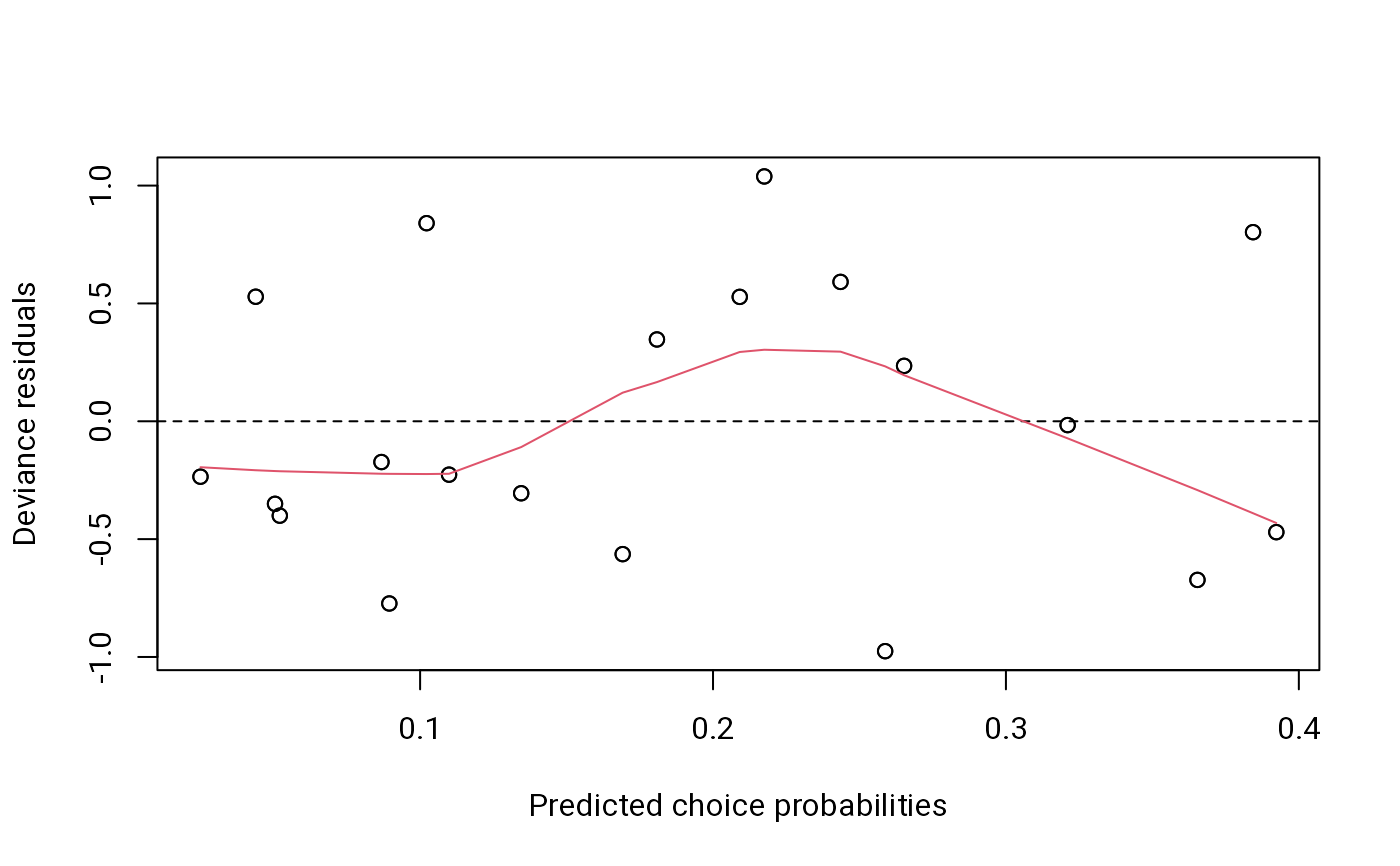
plot(ebao1)                    # residuals versus predicted values

confint(ebao1)                 # confidence intervals for parameters
#>             2.5 %     97.5 %
#> 1     0.008939213 0.01830734
#> 2     0.019689912 0.03675139
#> 3     0.048269446 0.08282664
#> 4     0.145905589 0.22482461
#> 5     0.346468731 0.44762381
#> order 1.110902126 1.56378025