World Valence and Source Memory for Vertical Position

Sixty-four participants studied words with positive, negative, or neutral valence displayed at the top or bottom part of a computer screen. Later, these words were presented intermixed with new words, and participants had to classify them as "top," "bottom," or "new." It was of interest if memory is improved in congruent trials, in which word valence and vertical position match (positive-top, negative-bottom), as opposed to incongruent trials.

data(valence)

Format

A data frame consisting of five components:

id

factor. Participant ID.

gender

factor. Participant gender.

age

participant age.

condition

factor. In congruent trials, positive words were presented at the top, negative words at the bottom, and vice versa for incongruent trials.

y

a matrix of aggregate response frequencies per participant and condition. The column names indicate each of nine response categories, for example, top.bottom means that words were presented at the top, but participant responded "bottom."

Source

Data were collected at the Department of Psychology, University of Tuebingen, in 2010.

See also

mpt.

Examples

data(valence)

## Fit source-monitoring model to subsets of data
spec <- mptspec("SourceMon", .restr=list(d1=d, d2=d))
names(spec$prob) <- colnames(valence$y)

mpt(spec, valence[valence$condition == "congruent" &
                  valence$gender == "female", "y"])
#> 
#> Multinomial processing tree (MPT) models
#> 
#> Parameter estimates:
#>     D1       d       g       b      D2  
#> 0.8463  0.5269  0.5131  0.1875  0.9038  
#> 
#> Goodness of fit (2 log likelihood ratio):
#> 	G2(1) = 0.0438, p = 0.8342
#> 
mpt(spec, valence[valence$condition == "incongruent" &
                  valence$gender == "female", "y"])
#> 
#> Multinomial processing tree (MPT) models
#> 
#> Parameter estimates:
#>     D1       d       g       b      D2  
#> 0.9281  0.3913  0.5873  0.1876  0.8698  
#> 
#> Goodness of fit (2 log likelihood ratio):
#> 	G2(1) = 1.836, p = 0.1754
#> 

## Test the congruency effect
val.agg <- aggregate(y ~ gender + condition, valence, sum)
y <- as.vector(t(val.agg[, -(1:2)]))

spec <- mptspec("SourceMon", .replicates=4,
                .restr=list(d11=d1, d21=d1, d12=d2, d22=d2,
                            d13=d3, d23=d3, d14=d4, d24=d4))
m1 <- mpt(spec, y)
m2 <- mpt(update(spec, .restr=list(d1=d.f, d3=d.f, d2=d.m, d4=d.m)), y)
anova(m2, m1)  # better discrimination in congruent trials
#> Analysis of Deviance Table
#> 
#> Model 1: m2
#> Model 2: m1
#>   Resid. Df Resid. Dev Df Deviance Pr(>Chi)   
#> 1         6     13.495                        
#> 2         4      3.570  2   9.9246 0.006997 **
#> ---
#> Signif. codes:  0 ‘***’ 0.001 ‘**’ 0.01 ‘*’ 0.05 ‘.’ 0.1 ‘ ’ 1

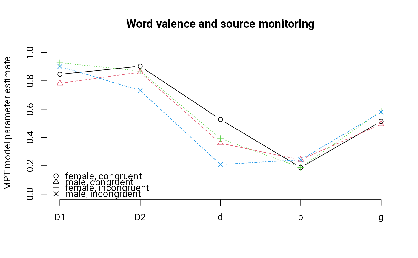
## Plot parameter estimates
mat <- matrix(coef(m1), 5)
rownames(mat) <- c("D1", "d",  "g",  "b",  "D2")
mat <- mat[c("D1", "D2", "d", "b", "g"), ]
matplot(mat, type="b", axes=FALSE, ylab="MPT model parameter estimate",
        main="Word valence and source monitoring", ylim=0:1, pch=1:4)
axis(1, 1:5, rownames(mat)); axis(2)
legend("bottomleft", c("female, congruent", "male, congruent",
       "female, incongruent", "male, incongruent"), pch=1:4, bty="n")