Wason Selection Task (WST) and Helpful Hints

In the Wason selection task, a participant is presented with four cards, each one having a letter side and a number side, e.g., A B 3 4. The task is to select the card(s) that have to be turned around in order to test the rule "If there is an A on the letter side then there is a 3 on the number side." Klauer, Stahl, and Erdfelder (2007) report a series of experiments to test their WST model using the aggregate frequencies of the 16 possible response patterns.

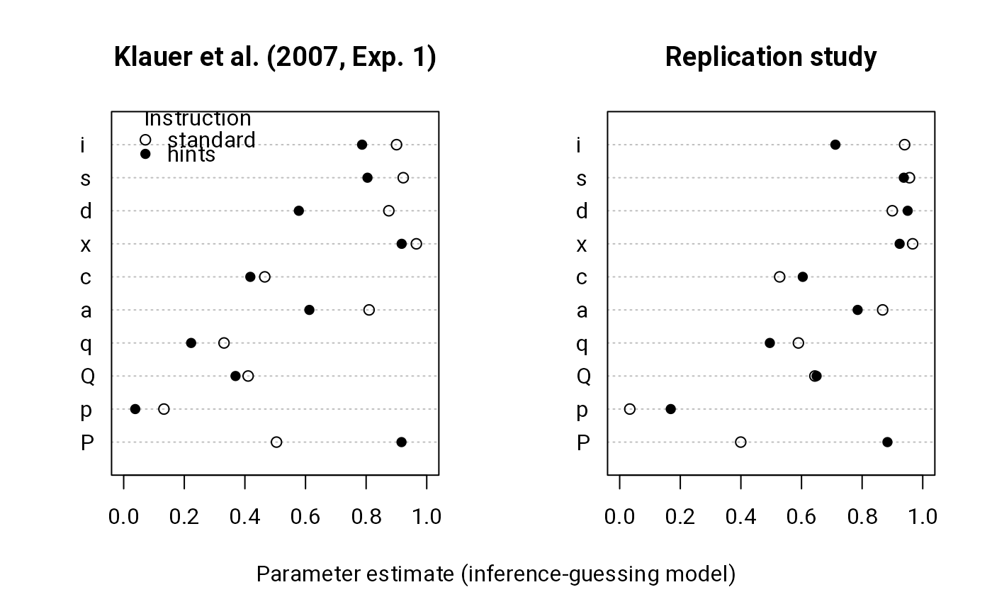
Bauder (2020) conducted a replication study that was designed to be similar to Experiment 1 in Klauer et al. (2007).

data(selectiontask)

Format

WSTKlauer2007 A data frame consisting of four variables:

group

factor. The control group (CG) received standard instructions, the experimental group (EG) got additional helpful hints.

pattern

character. Response pattern indicating which card(s) were selected (1) or not selected (0).

exp1, exp2

the aggregate response frequencies for Experiment 1 and 2, respectively.

WSTreplication A data frame containing 1118 observations of eight variables:

status

factor. Was the participant excluded?

group

factor. The experimental group.

gender

factor. Participant gender.

age

participant age.

education

years of education.

logic

factor. Familiarity with formal logic.

time

seconds spent on the web page.

y

a participant by response pattern indicator matrix.

Note

In the original analyses (Klauer et al., 2007), a constant of one was added to all frequencies.

Source

Klauer, K.C., Stahl, C., & Erdfelder, E. (2007). The abstract selection task: New data and an almost comprehensive model. Journal of Experimental Psychology: Learning, Memory, and Cognition, 33(4), 680--703. doi: 10.1037/0278-7393.33.4.680

Bauder, D. (2020). Die Modellierung der abstrakten Auswahlaufgabe von Wason - eine Replikationsstudie. Bachelor thesis. University of Tuebingen, Germany. https://osf.io/3z7ux/

See also

mpt.

Examples

data(selectiontask)

## Inference-guessing model with relaxed assumptions
s <- mptspec("WST", .replicates = 2)
m1 <- mpt(s, data = WSTKlauer2007$exp1, method = "EM")

## Inference-guessing model
m2 <- mpt(update(s, .restr = list(sf1=s1, sb1=s1, sfb1=s1,
                                  sf2=s2, sb2=s2, sfb2=s2)),
          data = m1$y, method = "EM")

## Effect of hint on i parameter (Exp. 1)
m3 <- mpt(update(m2$spec, .restr = list(i2=i1)), data = m1$y,
          method = "EM")

## Independence model
m4 <- mpt(update(m2$spec,
                 .restr = list(a1=0, c1=0, x1=0, d1=0, s1=0, i1=0,
                               a2=0, c2=0, x2=0, d2=0, s2=0, i2=0)),
          data = m1$y, method = "EM")

anova(m4, m3, m2, m1)
#> Analysis of Deviance Table
#> 
#> Model 1: m4
#> Model 2: m3
#> Model 3: m2
#> Model 4: m1
#>   Resid. Df Resid. Dev Df Deviance  Pr(>Chi)    
#> 1        22     320.29                          
#> 2        11      18.11 11  302.179 < 2.2e-16 ***
#> 3        10      10.21  1    7.902  0.004938 ** 
#> 4         6       6.67  4    3.535  0.472514    
#> ---
#> Signif. codes:  0 ‘***’ 0.001 ‘**’ 0.01 ‘*’ 0.05 ‘.’ 0.1 ‘ ’ 1
plogis(confint(m2))
#>                2.5 %    97.5 %
#> logit(a1) 0.68822950 0.8914302
#> logit(P1) 0.25347075 0.7528745
#> logit(p1) 0.03864804 0.3684090
#> logit(Q1) 0.20169925 0.6577479
#> logit(q1) 0.16203378 0.5589226
#> logit(c1) 0.39585065 0.5366287
#> logit(d1) 0.71963356 0.9501524
#> logit(s1) 0.86636088 0.9561735
#> logit(i1) 0.84887786 0.9356433
#> logit(x1) 0.87840983 0.9909880
#> logit(a2) 0.42783958 0.7699254
#> logit(P2) 0.78860486 0.9701727
#> logit(p2) 0.01017547 0.1327876
#> logit(Q2) 0.21958699 0.5488031
#> logit(q2) 0.12422896 0.3661908
#> logit(c2) 0.30618170 0.5387041
#> logit(d2) 0.33905302 0.7852455
#> logit(s2) 0.69073325 0.8834528
#> logit(i2) 0.69661269 0.8554926
#> logit(x2) 0.80280326 0.9679649
AIC(m2)
#> [1] 157.5821
BIC(m2)  # BIC w/number of non-redundant response categories
#> [1] 185.6061
AIC(m2, k = log(sum(m2$y)))  # BIC w/total number of data points
#> [1] 246.2088

## Effect of hint on c parameter (Exp. 2)
m5 <- mpt(m2$spec, data = WSTKlauer2007$exp2, method = "EM")
m6 <- mpt(update(m5$spec, .restr = list(c2=c1)), data = m5$y,
          method = "EM")
anova(m6, m5)
#> Analysis of Deviance Table
#> 
#> Model 1: m6
#> Model 2: m5
#>   Resid. Df Resid. Dev Df Deviance  Pr(>Chi)    
#> 1        11    26.6151                          
#> 2        10     8.3826  1   18.233 1.955e-05 ***
#> ---
#> Signif. codes:  0 ‘***’ 0.001 ‘**’ 0.01 ‘*’ 0.05 ‘.’ 0.1 ‘ ’ 1

## Replication of Exp. 1
wst.agg <- aggregate(y ~ group, WSTreplication,
                     subset = status == "select", sum)
y <- as.vector(t(wst.agg[, -1]))

set.seed(1503)
m7 <- mpt(m2$spec, data = y, start = runif(20), method = "EM")

idx <- c("P", "p", "Q", "q", "a", "c", "x", "d", "s", "i")
par(mfrow = 1:2)
dotchart(coef(m2)[paste0(idx, 1)], xlim=c(0, 1), labels=idx,
         main="Klauer et al. (2007, Exp. 1)", xlab="")
points(coef(m2)[paste0(idx, 2)], 1:10, pch=16)
legend(0, 11, c("standard", "hints"), pch=c(1, 16),
       title="Instruction", bty="n")
dotchart(coef(m7)[paste0(idx, 1)], xlim=c(0, 1), labels=idx,
         main="Replication study", xlab="")
points(coef(m7)[paste0(idx, 2)], 1:10, pch=16)
mtext("Parameter estimate (inference-guessing model)", side=1,
      outer=TRUE, line=-2)