Diagnostic Plot for MPT Models

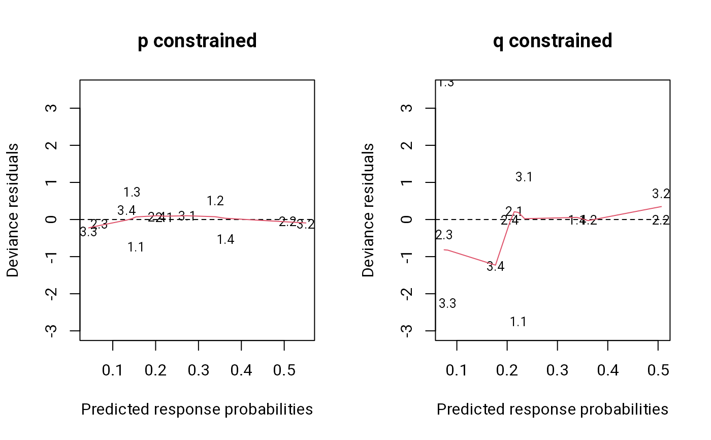
Plots MPT residuals against fitted values.

# S3 method for mpt
plot(x, showNames = TRUE,
     xlab = "Predicted response probabilities", ylab = "Deviance residuals",
     ...)

# S3 method for mpt
residuals(object, type = c("deviance", "pearson"), ...)

Arguments

x, object

an object of class mpt, typically the result of a call to mpt.

showNames

logical. Should the names of the residuals be plotted? Defaults to TRUE.

xlab, ylab

graphical parameters passed to plot.

type

the type of residuals which should be returned; the alternatives are: "deviance" (default) and "pearson".

...

further arguments passed to or from other methods.

Details

The deviance residuals are plotted against the predicted response probabilities. If showNames is true, plotting symbols are the names of the residuals.

Value

For residuals, a named vector of residuals having as many elements as response categories.

See also

mpt, residuals.glm.

Examples

## Compare two constrained MPT models
data(proact)

spec <- mptspec(
  p1*q1*r1,
  p1*q1*(1 - r1),
  p1*(1 - q1)*r1,
  (1 - p1) + p1*(1 - q1)*(1 - r1),

  p2*q2*r2,
  p2*q2*(1 - r2),
  p2*(1 - q2)*r2,
  (1 - p2) + p2*(1 - q2)*(1 - r2),

  p3*q3*r3,
  p3*q3*(1 - r3),
  p3*(1 - q3)*r3,
  (1 - p3) + p3*(1 - q3)*(1 - r3)
)
m1 <- mpt(update(spec, .restr = list(p2=p1, p3=p1)),
          proact[proact$test == 1, ])
m2 <- mpt(update(spec, .restr = list(q2=q1, q3=q1)), m1$y)

par(mfrow = c(1, 2))                 # residuals versus fitted values
plot(m1, main = "p constrained", ylim = c(-3, 3.5))  # good fit
plot(m2, main = "q constrained", ylim = c(-3, 3.5))  # bad fit


sum( resid(m1)^2 )                   # likelihood ratio G2
#> [1] 1.845292
sum( resid(m1, "pearson")^2 )        # Pearson X2
#> [1] 1.845037