Quality of Multichannel Reproduced Sound
soundquality.RdPaired comparison judgments of 40 selected listeners with respect to
eight audio reproduction modes and four types of music:
SQpreference includes judgments on overall preference;
SQattributes includes judgments on specific spatial and timbral
auditory attributes;
SQsubjects: includes information about the listeners involved.
data("soundquality")Format
SQpreference A data frame containing 783 observations on 6 variables:
- id
factor, listener ID.
- time
factor, listening experiment before or after elicitation and scaling of more specific auditory attributes.
- progmat
factor, the program material: Beethoven, Rachmaninov, Steely Dan, Sting.
- repet
the repetition number.
- session
the experimental session coding the presentation order of the program material.
- preference
paired comparison of class
paircomp; preferences for all 28 paired comparisons from 8 audio reproduction modes: Mono, Phantom Mono, Stereo, Wide-Angle Stereo, 4-channel Matrix, 5-channel Upmix 1, 5-channel Upmix 2, and 5-channel Original.
SQattributes A data frame containing 156 observations on 10 variables:
- id
factor, listener ID.
- progmat
factor, the program material.
- width, spaciousness, envelopment, distance, clarity, brightness, elevation, naturalness
Paired comparison of class
paircomp.
SQsubjects A data frame containing 78 observations on 18 variables:
- id
factor, listener ID
- status
factor, selection status; 40 listeners were selected.
- HLmax
maximum hearing level between 250 and 8000 Hz
- stereowidth
stereo-width discrimination threshold
- fluency
word fluency score
- age
subject age
- gender
factor, subject gender
- education
factor, education class
- background, experience, listenmusic, concerts, instrument, critical, cinema, hifi, surround, earliertests
indicators of prior experience
Details
The data were collected within a series of experiments conducted at the Sound Quality Research Unit (SQRU), Department of Acoustics, Aalborg University, Denmark, between September 2004 and March 2005.
The results of scaling listener preference and spatial and timbral auditory attributes are reported in Choisel and Wickelmaier (2007). See examples for replication code. Details about the loudspeaker setup and calibration are given in Choisel and Wickelmaier (2006). The attribute elicitation procedure is described in Wickelmaier and Ellermeier (2007) and in Choisel and Wickelmaier (2006). The selection of listeners for the experiments is described in Wickelmaier and Choisel (2005).
Portions of these data are also available via data("SoundQuality",
package = "psychotools").
Note
One listener (ID 62) dropped out after contributing the first set of preference judgments.
References
Choisel, S., & Wickelmaier, F. (2006). Extraction of auditory features and elicitation of attributes for the assessment of multichannel reproduced sound. Journal of the Audio Engineering Society, 54(9), 815–826.
Choisel, S., & Wickelmaier, F. (2007). Evaluation of multichannel reproduced sound: Scaling auditory attributes underlying listener preference. Journal of the Acoustical Society of America, 121(1), 388–400. doi:10.1121/1.2385043
Wickelmaier, F., & Choisel, S. (2005). Selecting participants for listening tests of multichannel reproduced sound. Presented at the AES 118th Convention, May 28–31, Barcelona, Spain, convention paper 6483.
Wickelmaier, F., & Ellermeier, W. (2007). Deriving auditory features from triadic comparisons. Perception & Psychophysics, 69(2), 287–297. doi:10.3758/BF03193750
Examples
requireNamespace("psychotools")
data(soundquality)
######### Replication code for Choisel and Wickelmaier (2007) ######
### A. Scaling overall preference
## Participants
summary(subset(SQsubjects, status == "selected"))
#> id status HLmax stereowidth fluency
#> 04 : 1 rejected: 0 Min. :10.00 Min. :0.4586 Min. :13.00
#> 05 : 1 selected:40 1st Qu.:15.00 1st Qu.:0.5310 1st Qu.:15.00
#> 07 : 1 Median :15.00 Median :0.6173 Median :18.50
#> 08 : 1 Mean :15.75 Mean :0.6137 Mean :17.95
#> 10 : 1 3rd Qu.:20.00 3rd Qu.:0.7112 3rd Qu.:20.25
#> 11 : 1 Max. :20.00 Max. :0.7640 Max. :29.00
#> (Other):34
#> age gender education background experience
#> Min. :21.00 female:12 < 10 : 2 music : 9 no :26
#> 1st Qu.:23.00 male :28 10 to 13: 1 engineering:17 yes:14
#> Median :24.00 13 to 16:17 languages : 5
#> Mean :25.18 > 16 :20 socialsci : 7
#> 3rd Qu.:26.25 other : 2
#> Max. :39.00
#>
#> listenmusic concerts instrument critical cinema hifi surround
#> weekly: 5 no : 3 no :10 no : 3 no : 1 no : 7 no :33
#> daily :35 rarely :16 rarely: 5 yes:37 rarely :17 yes:33 yes: 7
#> monthly:15 weekly: 9 monthly:22
#> weekly : 6 daily :16 weekly : 0
#>
#>
#>
#> earliertests
#> no :26
#> yes:14
#>
#>
#>
#>
#>
## Transitivity violations
aggregate(preference ~ progmat + time,
data = SQpreference,
function(x) unlist(strans(summary(x, pcmatrix = TRUE))[
c("weak", "moderate", "strong")]))
#> progmat time mf[[1L]].weak mf[[1L]].moderate mf[[1L]].strong
#> 1 Beethoven before 0 2 14
#> 2 Rachmaninov before 2 4 19
#> 3 SteelyDan before 0 0 12
#> 4 Sting before 0 0 13
#> 5 Beethoven after 0 1 12
#> 6 Rachmaninov after 0 0 18
#> 7 SteelyDan after 0 0 11
#> 8 Sting after 0 0 9
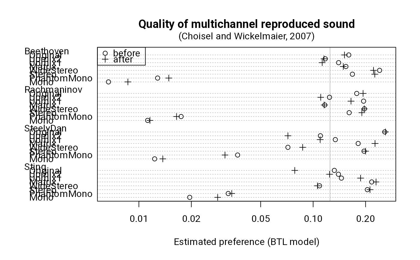
## BTL modeling
prefdf <- aggregate(preference ~ progmat + time,
data = SQpreference,
function(x) uscale(eba(summary(x, pcmatrix = TRUE))))
## Preference scale
p <- t(prefdf[prefdf$time == "before", 3])
colnames(p) <- levels(prefdf$progmat)
dotchart(p, main = "Quality of multichannel reproduced sound",
xlab = "Estimated preference (BTL model)", log = "x",
panel.first = abline(v = 1/8, col = "gray"))
points(x = t(prefdf[prefdf$time == "after", 3]),
y = c(31:38, 21:28, 11:18, 1:8), pch = 3)
legend("topleft", c("before", "after"), pch = c(1, 3))
mtext("(Choisel and Wickelmaier, 2007)", line = 0.5)
 ### B. Scaling specific auditory attributes
## Transitivity violations
aggregate(
x = SQattributes[-(1:2)],
by = list(progmat = SQattributes$progmat),
FUN = function(x) strans(summary(x, pcmatrix = TRUE))[
c("weak", "moderate", "strong")],
simplify = FALSE
)
#> progmat width spaciousness envelopment distance clarity brightness
#> 1 Beethoven 0, 1, 19 0, 2, 18 0, 3, 23 3, 9, 32 4, 5, 27 2, 3, 19
#> 2 Rachmaninov 1, 1, 14 2, 7, 19 2, 4, 27 2, 11, 37 2, 6, 21 4, 4, 27
#> 3 SteelyDan 0, 3, 14 2, 2, 19 0, 2, 23 3, 13, 30 0, 2, 18 0, 0, 15
#> 4 Sting 0, 2, 24 0, 4, 16 1, 3, 16 0, 1, 19 2, 3, 16 0, 0, 23
#> elevation naturalness
#> 1 1, 11, 25 3, 5, 24
#> 2 2, 7, 23 0, 2, 14
#> 3 0, 2, 24 0, 2, 18
#> 4 0, 0, 16 1, 1, 18
## BTL modeling
uscal <- aggregate(
x = SQattributes[-(1:2)],
by = list(progmat = SQattributes$progmat),
FUN = function(x) uscale(eba(summary(x, pcmatrix = TRUE)))
)
uscal <- data.frame(
progmat = rep(levels(SQattributes$progmat), each = 8),
repmod = factor(1:8, labels = labels(SQattributes$width)),
as.data.frame(sapply(uscal[-1], t))
)
## EBA modeling: envelopment, width
uscal$envelopment[uscal$progmat == "SteelyDan"] <-
uscale(eba(summary(SQattributes[SQattributes$progmat == "SteelyDan",
"envelopment"], pcmatrix = TRUE),
A = list(c(1,9), c(2,9), c(3,9), c(4,9), 5, 6, c(7,9), 8)))
uscal$width[uscal$progmat == "SteelyDan"] <-
uscale(eba(summary(SQattributes[SQattributes$progmat == "SteelyDan",
"width"], pcmatrix = TRUE),
A = list(1, 2, c(3,9), c(4,9), c(5,9), 6, 7, c(8,9))))
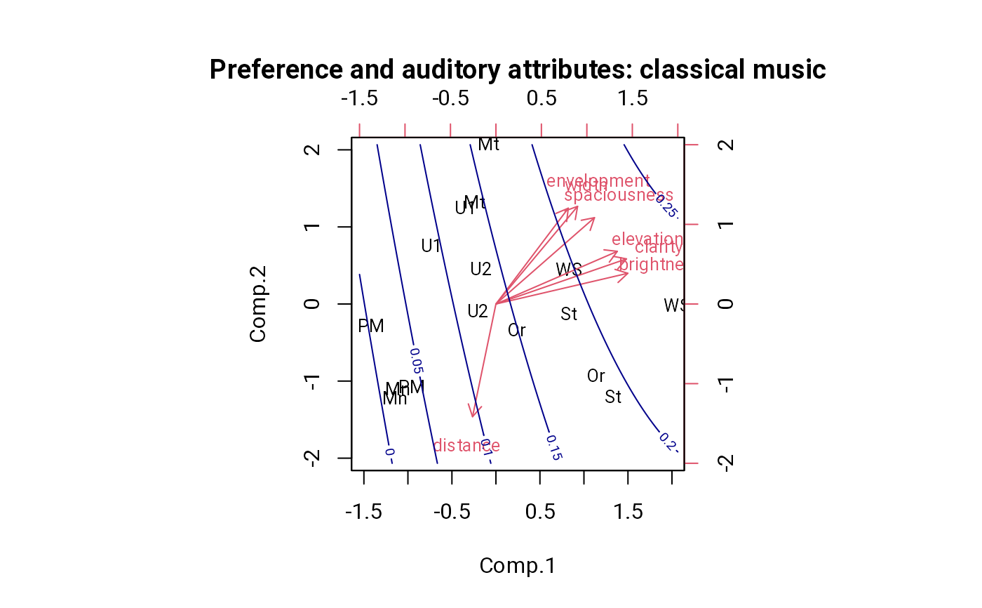
### C. Relating overall preference to specific attributes
## Principal components: classical music
pca1 <- princomp(
~ width + spaciousness + envelopment + distance +
clarity + brightness + elevation,
data = uscal,
subset = progmat %in% c("Beethoven", "Rachmaninov"),
cor = TRUE
)
## Loadings on first two components
L <- varimax(loadings(pca1) %*% diag(pca1$sdev)[, 1:2])
## Factor scores
f <- scale(predict(pca1)[, 1:2]) %*% L$rotmat
dimnames(f) <- list(
abbreviate(rep(labels(SQattributes$width), 2), 2),
names(pca1$sdev)[1:2]
)
biplot(f, 2*L$loadings, cex = 0.8, expand = 1.5,
main = "Preference and auditory attributes: classical music",
xlim = c(-1.5, 2), ylim = c(-2, 2))
## Predicting preference
classdf <- cbind(
pref = as.vector(t(prefdf[prefdf$time == "after" &
prefdf$progmat %in% c("Beethoven", "Rachmaninov"), 3])),
as.data.frame(f)
)
m1 <- lm(pref ~ Comp.1 + Comp.2 + I(Comp.1^2), classdf)
c1 <- seq(-1.5, 2.0, length.out = 101)
c2 <- seq(-2.0, 2.0, length.out = 101)
z <- matrix(predict(m1, expand.grid(Comp.1 = c1, Comp.2 = c2)), 101, 101)
contour(c1, c2, z, add = TRUE, col = "darkblue")
### B. Scaling specific auditory attributes
## Transitivity violations
aggregate(
x = SQattributes[-(1:2)],
by = list(progmat = SQattributes$progmat),
FUN = function(x) strans(summary(x, pcmatrix = TRUE))[
c("weak", "moderate", "strong")],
simplify = FALSE
)
#> progmat width spaciousness envelopment distance clarity brightness
#> 1 Beethoven 0, 1, 19 0, 2, 18 0, 3, 23 3, 9, 32 4, 5, 27 2, 3, 19
#> 2 Rachmaninov 1, 1, 14 2, 7, 19 2, 4, 27 2, 11, 37 2, 6, 21 4, 4, 27
#> 3 SteelyDan 0, 3, 14 2, 2, 19 0, 2, 23 3, 13, 30 0, 2, 18 0, 0, 15
#> 4 Sting 0, 2, 24 0, 4, 16 1, 3, 16 0, 1, 19 2, 3, 16 0, 0, 23
#> elevation naturalness
#> 1 1, 11, 25 3, 5, 24
#> 2 2, 7, 23 0, 2, 14
#> 3 0, 2, 24 0, 2, 18
#> 4 0, 0, 16 1, 1, 18
## BTL modeling
uscal <- aggregate(
x = SQattributes[-(1:2)],
by = list(progmat = SQattributes$progmat),
FUN = function(x) uscale(eba(summary(x, pcmatrix = TRUE)))
)
uscal <- data.frame(
progmat = rep(levels(SQattributes$progmat), each = 8),
repmod = factor(1:8, labels = labels(SQattributes$width)),
as.data.frame(sapply(uscal[-1], t))
)
## EBA modeling: envelopment, width
uscal$envelopment[uscal$progmat == "SteelyDan"] <-
uscale(eba(summary(SQattributes[SQattributes$progmat == "SteelyDan",
"envelopment"], pcmatrix = TRUE),
A = list(c(1,9), c(2,9), c(3,9), c(4,9), 5, 6, c(7,9), 8)))
uscal$width[uscal$progmat == "SteelyDan"] <-
uscale(eba(summary(SQattributes[SQattributes$progmat == "SteelyDan",
"width"], pcmatrix = TRUE),
A = list(1, 2, c(3,9), c(4,9), c(5,9), 6, 7, c(8,9))))
### C. Relating overall preference to specific attributes
## Principal components: classical music
pca1 <- princomp(
~ width + spaciousness + envelopment + distance +
clarity + brightness + elevation,
data = uscal,
subset = progmat %in% c("Beethoven", "Rachmaninov"),
cor = TRUE
)
## Loadings on first two components
L <- varimax(loadings(pca1) %*% diag(pca1$sdev)[, 1:2])
## Factor scores
f <- scale(predict(pca1)[, 1:2]) %*% L$rotmat
dimnames(f) <- list(
abbreviate(rep(labels(SQattributes$width), 2), 2),
names(pca1$sdev)[1:2]
)
biplot(f, 2*L$loadings, cex = 0.8, expand = 1.5,
main = "Preference and auditory attributes: classical music",
xlim = c(-1.5, 2), ylim = c(-2, 2))
## Predicting preference
classdf <- cbind(
pref = as.vector(t(prefdf[prefdf$time == "after" &
prefdf$progmat %in% c("Beethoven", "Rachmaninov"), 3])),
as.data.frame(f)
)
m1 <- lm(pref ~ Comp.1 + Comp.2 + I(Comp.1^2), classdf)
c1 <- seq(-1.5, 2.0, length.out = 101)
c2 <- seq(-2.0, 2.0, length.out = 101)
z <- matrix(predict(m1, expand.grid(Comp.1 = c1, Comp.2 = c2)), 101, 101)
contour(c1, c2, z, add = TRUE, col = "darkblue")
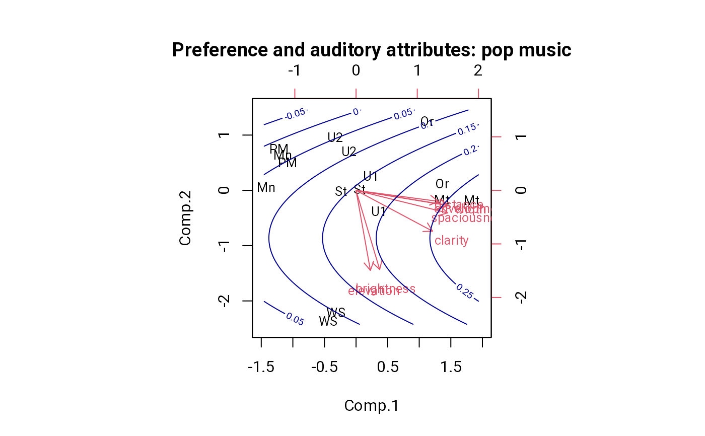
 ## Principal components: pop music
pca2 <- princomp(
~ width + spaciousness + envelopment + distance +
clarity + brightness + elevation,
data = uscal,
subset = progmat %in% c("SteelyDan", "Sting"),
cor = TRUE
)
L <- varimax(loadings(pca2) %*% diag(pca2$sdev)[, 1:2])
f[] <- scale(predict(pca2)[, 1:2]) %*% L$rotmat
biplot(f, 2*L$loadings, cex = 0.8,
main = "Preference and auditory attributes: pop music",
xlim = c(-1.5, 2), ylim = c(-2.5, 1.5))
popdf <- cbind(
pref = as.vector(t(prefdf[prefdf$time == "after" &
prefdf$progmat %in% c("SteelyDan", "Sting"), 3])),
as.data.frame(f)
)
m2 <- lm(pref ~ Comp.1 + Comp.2 + I(Comp.2^2), popdf)
c1 <- seq(-1.5, 2.0, length.out = 101)
c2 <- seq(-2.5, 1.5, length.out = 101)
z <- matrix(predict(m2, expand.grid(Comp.1 = c1, Comp.2 = c2)), 101, 101)
contour(c1, c2, z, add = TRUE, col = "darkblue")
## Principal components: pop music
pca2 <- princomp(
~ width + spaciousness + envelopment + distance +
clarity + brightness + elevation,
data = uscal,
subset = progmat %in% c("SteelyDan", "Sting"),
cor = TRUE
)
L <- varimax(loadings(pca2) %*% diag(pca2$sdev)[, 1:2])
f[] <- scale(predict(pca2)[, 1:2]) %*% L$rotmat
biplot(f, 2*L$loadings, cex = 0.8,
main = "Preference and auditory attributes: pop music",
xlim = c(-1.5, 2), ylim = c(-2.5, 1.5))
popdf <- cbind(
pref = as.vector(t(prefdf[prefdf$time == "after" &
prefdf$progmat %in% c("SteelyDan", "Sting"), 3])),
as.data.frame(f)
)
m2 <- lm(pref ~ Comp.1 + Comp.2 + I(Comp.2^2), popdf)
c1 <- seq(-1.5, 2.0, length.out = 101)
c2 <- seq(-2.5, 1.5, length.out = 101)
z <- matrix(predict(m2, expand.grid(Comp.1 = c1, Comp.2 = c2)), 101, 101)
contour(c1, c2, z, add = TRUE, col = "darkblue")